Dimensionality Reduction and Principal Component Analysis

Dimensionality Reduction and Principal Component Analysis –

What is Dimensionality reduction –

First, we will discuss about the dimensionality when we take any dataset for the processing or to apply the model then in that number of features, variables or columns are present as input features. All these input features are called as dimensionality. The method to reduce this input features are called as dimensionality reduction. The dataset contains vary large number of input variables to make the predictive analysis but this huge number of features makes prediction more complicated. This is because if the input variables are in more numbers, then it is difficult to visualize the data during training to overcome this, we need to do the dimensionality reduction. 

Another way we can define dimensionality reduction is to convert dataset with higher dimension to a smaller number of dimensions by providing the similar information. Dimensionality reduction can be used for classification as well as regression problems in machine learning. This technique can be used to deal with larger dimensional dataset like speech recognition, signal processing etc. Also, we can use dimensionality reduction for noise reduction, clustering analysis, and data visualization. 

For Free, Demo classes Call:  8983120543

Registration Link: Click Here!

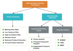
Basically, dimensionality reduction techniques are divided into the two classes like feature selection and dimensionality reduction. The feature selection will consider the following points like filter for low variance and high correlation, missing value ratio, forward feature selection and backward feature extraction. The dimensionality reduction is again divided into two classes such as component or feature based and project based. The feature-based class will consider the following points like principal component analysis, factor analysis etc. the project-based class will consist of ISOMAP, UMAP, t-SNE etc.  

 

It is very difficult in practice to handle the high dimensional data such a condition is known as curse of dimensionality. As the input features are increased then it is very complex to apply any machine learning algorithm or to make a model. If a machine learning model is applied on such noise data or high dimensional data then chances of overfitting will be high. If the model is trained on such data, then it will get poor results. So, to avoid this we need to do the dimensionality reduction. 

Advantages of Dimensionality Reduction

1. Less time is required to train the model. 
2. Also, less memory is required to store the dataset.
3. It is very easy to remove the redundant features if available in the dataset by using multicollinearity. 
4. We can visualize the data very quickly. 

Disadvantages of Dimensionality Reduction

1. When we use principal component analysis for dimensionality reduction then we need to consider some points to be unknown. 
2. During dimensionality reduction some data may be lost.

The principal component analysis, high correlation, missing value ratio, backward elimination, forward selection, low variance filter, score comparison, factor analysis etc are the various techniques used for dimensionality reduction. Here we will discuss more about the principal component analysis.  

Principal Component Analysis  

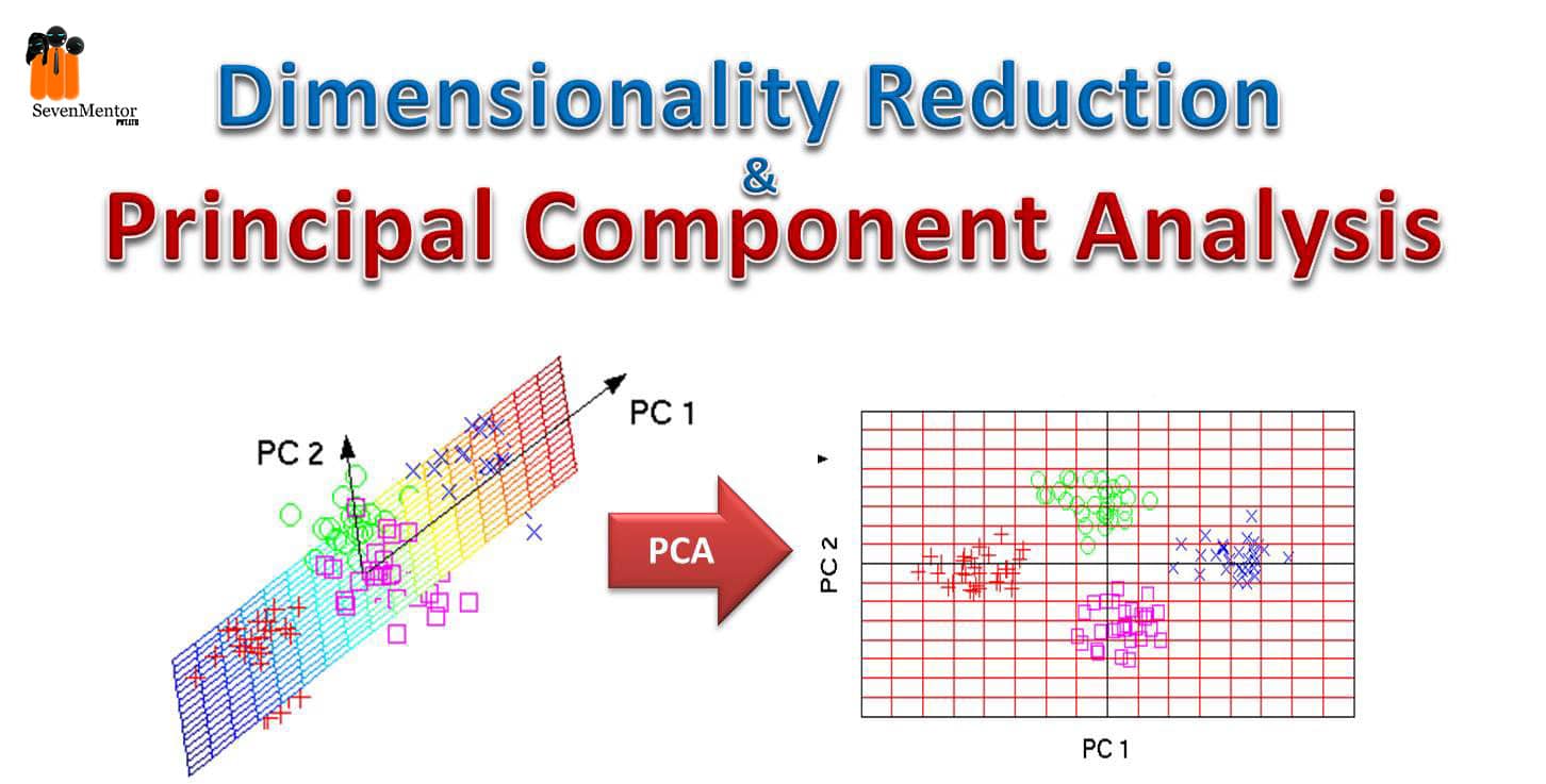
Principal component analysis is an unsupervised machine learning algorithm and this is used for dimensionality reduction. In this process by using orthogonal transformation convert the observation of correlated features into a linearly uncorrelated feature set and this new feature is known as the principal component. This is the most popular technique used for predictive modelling, data analysis, also used to identify the strong pattern from a given dataset by reducing the variance. The principal component analysis is mostly used for movie recommendation systems, image processing etc. In principal component analysis many mathematical concepts are used such as variance and covariance, eigenvalues and eigenvectors. 

For Free, Demo classes Call:  8983120543

Registration Link: Click Here!

Common Terms in Principal Component Analysis 

1. Dimensionality: In the given dataset number of variables or features are present that is called dimension. We can say in other words like the number of columns present in the dataset is known as dimension of dataset. 
2. Correlation: this term defines the relationship between two variables. It defines how strongly two variables are related to each other. So, we can say that if one variable changes then automatically the second will change. The value of correlation is in between -1 to +1. If this correlation value is -1 then two variables are not related with each other or we can say that are inversely proportional to each other. If the correlation value is +1 then two variables are strongly related to each other or we can say that these two variables are directly proportional to each other. 
3. Orthogonal: when the two variables are not related to each other and correlation value is zero. 
4. Eigenvector: If the non-zero vector and square matrix is given then the non-zero vector will be the eigenvector. 
5. Covariance matrix: If the covariance between the two pairs of variables is given in a matrix, then the matrix is called a covariance matrix.

Steps in Principal Component Analysis:

1. The first step in any machine learning model is to get the input dataset. After getting the data we need to visualize the data and do the preprocessing like remove the null values, remove the outliers etc. After this we need to divide the dataset in the two groups like X and Y, X will be the training data and Y will be the testing or we can say validation dataset.
2. After that we need to structure the dataset into a two- dimensional matrix of independent variable X. When we structure the data, each row corresponding to data is variable and each column will represent the feature of the dataset. The number of columns present in the dataset will give us the dimension of the dataset.
3. After this we will use the standard scaler method to standardize our dataset because here high variance variables will be compared with low variance variables. To avoid this, we will do the standardization. 

From sklearn.preprocessing import StandardScaler

X = StandardScaler().fit_transform(X)

1. Then we will calculate the covariance of the variable and output will be in the covariance matrix (Z).

Mean=np.mean(X, axis=0)

Covariancematrix=(X-mean).T.dot((X-mean)) / (X.shape[0]-1)

Covariancematrix=np.cov(X.T)

1. Also, we will calculate the eigenvalue and eigenvector. 

Eigenvalues, eigenvector = np.linalg.eif(cov_mat)

1. After calculating the eigenvalues and vectors we will sort them in decreasing order from lowest to highest. The output will get in matrix (P)
2. Now the next step is to calculate new features by calculating the matrix P by Z. The output will be given in resultant matrix Z*
3. The last step is to remove the unimportant features from the dataset. So only we will keep the important features in the new dataset. 

For Free, Demo classes Call:  8983120543

Registration Link: Click Here!

Author:-

| SevenMentor Pvt Ltd.

© Copyright 2021 | Sevenmentor Pvt Ltd.