THE STORY OF DIMENSION REDUCTION…  

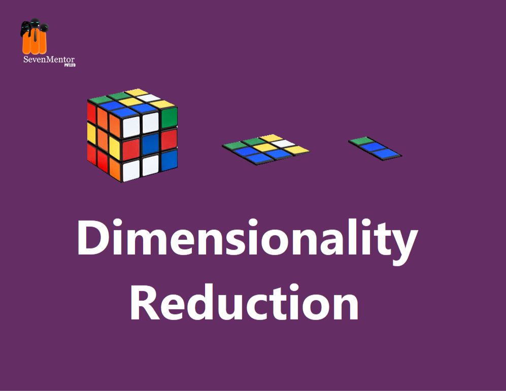
Dimension reduction is a common data preprocessing technique used in machine learning and data analysis. It involves reducing the number of variables or features in a dataset while retaining as much information as possible. This is done to simplify the analysis process, increase computational efficiency, and improve the accuracy of the model. In this blog, we will discuss the different techniques used for dimension reduction.  

Principal Component Analysis (PCA) 

 

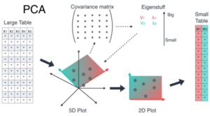
PCA is one of the most commonly used dimensionality reduction techniques. It is a linear transformation technique that converts a set of correlated variables into a set of uncorrelated variables called principal components. The first principal component accounts for the most variance in the data, while the subsequent principal components account for the remaining variance in descending order.

 

For Free, Demo classes Call: 7507414653
Registration Link: Click Here!

  

PCA works by identifying the directions of maximum variance in the data and projecting the data onto these directions. The principal components are then obtained as linear combinations of the original variables. PCA is used extensively in image processing, bioinformatics, finance, and many other areas.  

If you’re looking to break into the exciting and rapidly-growing field of Machine Learning, look no further than SevenMentor’s Machine Learning classes in Pune! Our comprehensive courses cover everything you need to know to get started with Machine Learning

PCA is based on the mathematical concept of eigenvectors and eigenvalues. Given a matrix A, an  eigenvector v and its corresponding eigenvalue λ satisfy the equation:  

Av = λv 

In PCA, we start with a matrix X containing n observations of p variables. We center the data by  subtracting the mean from each variable, giving us a matrix Z. We then calculate the covariance  matrix C of Z:  

C = Z^T Z / (n—1)

The covariance matrix measures how the variables in the dataset are related to each other. It is a  symmetric matrix, so it has a set of p eigenvectors that are orthogonal to each other.  

We then calculate the eigenvalues and eigenvectors of C. The eigenvectors are the principal components of the dataset, and the corresponding eigenvalues represent the amount of variance explained by each principal component.  

 

For Free, Demo classes Call: 7507414653
Registration Link: Click Here!

 

We can then project the data onto the principal components by multiplying the matrix Z by the matrix of eigenvectors. This gives us a new matrix Y, where each row represents an observation and each column represents a principal component.  

 

t-Distributed Stochastic Neighbour Embedding (t-SNE) 

 

t-SNE (t-Distributed Stochastic Neighbour Embedding) is a popular machine learning algorithm used for visualizing high-dimensional data in a low-dimensional space. It was introduced by  Laurens van der Maaten and Geoffrey Hinton in 2008.  

The t-SNE algorithm works by taking a set of high-dimensional data points and mapping them to a  low-dimensional space, typically two or three dimensions, in such a way that similar points in the 

high-dimensional space is mapped close together in the low-dimensional space, while dissimilar points are mapped far apart.  

The algorithm works by first constructing a probability distribution over pairs of high-dimensional data points, such that similar points have a higher probability of being chosen. It then constructs a  similar probability distribution over pairs of points in the low-dimensional space and tries to minimize the difference between the two distributions using gradient descent.  

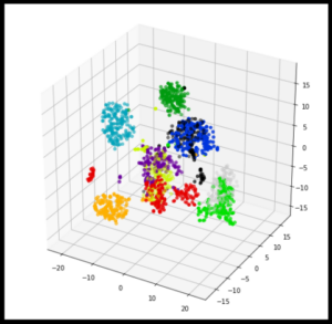
t-SNE is often used for data visualization tasks such as clustering and dimensionality reduction and has been applied to a wide range of fields including biology, computer vision, and natural language processing.  

The t-SNE algorithm involves several mathematical steps. Here is a brief summary of the main  calculations involved:  

1. Calculation of pairwise similarities: Given a high-dimensional dataset, t-SNE first calculates  the pairwise similarities between data points using a Gaussian kernel: 

p_{j|i} = exp(- ||x_i—x_j||² / 2sigma_i²) / sum(exp(- ||x_i—x_k||² / 2sigma_i²)) where p_{j|i} is the probability of choosing data point j as a neighbor of data point i, and  sigma_i is a parameter that controls the width of the Gaussian kernel for each data point.  2. Calculation of pairwise similarities in the low-dimensional space: t-SNE then constructs a  similar probability distribution over pairs of points in the low-dimensional space using a  Student t-distribution: 

q_{j|i} = (1 + ||y_i—y_j||²)^-1 / sum(1 + ||y_i—y_k||²)^-1 

where q_{j|i} is the probability of choosing data point j as a neighbor of data point I in the low-dimensional space, and y_i is the low-dimensional representation of data point i.  3. Optimisation: t-SNE then minimizes the difference between the two probability distributions using gradient descent. The cost function used is the Kullback-Leibler (KL) divergence  between the two distributions: 

KL(P||Q) = sum_{i!=j} p_{j|i} log(p_{j|i} / q_{j|i}) 

t-SNE minimizes this cost function with respect to the low-dimensional representation y_i  using gradient descent.  

 

For Free, Demo classes Call: 7507414653
Registration Link: Click Here!

 

4. Tuning of hyper-parameters: t-SNE also involves tuning of hyper-parameters such as the perplexity, which controls the balance between local and global structure in the data, and the learning rate, which controls the step size in the optimization process.  

Overall, t-SNE is a powerful technique for visualizing high-dimensional data, but its mathematical complexity can make it challenging to implement and interpret. 

 

Author: